5.1 Count Features in Samples

To count the number of features identified in each sample, we use colSums to tally the number of entries that are not NA in each column of exprs(oca.set).

# Calculate the number of proteins identified (not NA) in each sample
oca.set$num_proteins <- colSums(!is.na(exprs(oca.set)))

Now that we have a vector of the number of proteins detected in each sample stored in pData(oca.set), there are a few ways to present it. The first is a simple summary, which is accomplished with the summary function. This outputs the average value, as well as a 5-number summary that includes the minimum, the 1st quartile, the median (2nd quartile), the 3rd quartile, and the maximum value.

summary(oca.set$num_proteins)

##    Min. 1st Qu.  Median    Mean 3rd Qu.    Max. 
##    6594    6957    7286    7225    7463    7798

The 5-number summary can also be presented as a boxplot, which is typically more useful at a glance. Below is an example of how to create a horizontal boxplot.

# Horizontal boxplot
boxplot(oca.set$num_proteins, horizontal = TRUE,
        xlab = "Number of Proteins Detected")

Boxplots are useful, but a lot of the finer details about the distribution are lost when summarizing. To remedy this, we could instead show a scatterplot of the individual values with the base plot function. We will change the point type with pch to plot solid circles and change the axis titles with xlab and ylab.

plot(oca.set$num_proteins, pch = 19, xlab = "Sample Index", 
     ylab = "Number of Proteins Detected")

While harder to interpret at a glance than a boxplot, scatterplots are useful for identifying potential outliers and possible trends in the data. In the plot above, it doesn’t appear than there are any samples with significantly fewer identifications.

The other plot type we could use balances the summary of the boxplot with the finer detail of the scatterplot: kernel density plots. We can use a combination of stats::density and base::plot to quickly create a density plot.

# Kernel density plot
plot(density(oca.set$num_proteins, na.rm = TRUE), 
     xlim = range(oca.set$num_proteins, na.rm = TRUE),
     main = "Density Plot", xlab = "Number of Proteins Detected")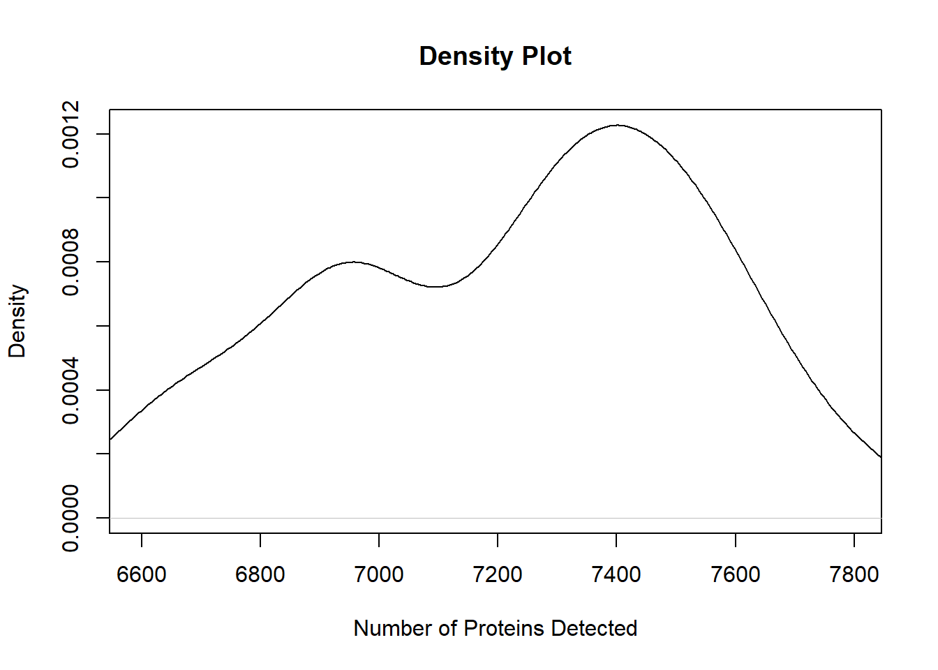

It looks like there are peaks around 6900-7000 and 7300-7500 proteins.