7.1 Linear Regression
limma_a_b or limma_gen are used to perform linear regression, which models the linear relationship between a numeric predictor and the feature-wise values in the exprs slot of an MSnSet.
For this example, we will test the AGE column of pData(m). The model.str is the full model that includes the variable of interest and any covariates. The coef.str argument is the variable of interest.
lm_res <- limma_gen(m, model.str = "~ AGE", coef.str = "AGE")
head(arrange(lm_res, adj.P.Val)) # top 6 rows sorted by adjusted p-value
## logFC AveExpr t P.Value adj.P.Val
## NP_001077077.1 -0.10468905 -4.163336e-17 -4.186740 0.0001865011 0.5982300
## NP_001138679.1 0.01185948 7.806256e-18 3.821284 0.0002953129 0.5982300
## NP_003286.1 0.01335415 -6.938894e-18 3.870673 0.0002292102 0.5982300
## NP_055336.1 -0.01819954 1.233581e-18 -3.986807 0.0002306581 0.5982300
## NP_000026.2 -0.01689006 -5.703200e-18 -2.847600 0.0056747708 0.8201268
## NP_000176.2 -0.02059760 -3.802134e-18 -3.055901 0.0031033317 0.8201268
## B
## NP_001077077.1 0.001863506
## NP_001138679.1 -1.049384099
## NP_003286.1 -0.880645496
## NP_055336.1 -0.598496581
## NP_000026.2 -3.895795433
## NP_000176.2 -3.338485703The logFC column is the slope of the regression line, and the AveExpr column is the average of the values for that feature (same as rowMeans(exprs(m), na.rm = TRUE)). AveExpr can also be thought of as the y-intercept of the regression line when the predictor is mean-centered. The actual y-intercept is \(\text{AveExpr} - avg(\text{AGE})\cdot\text{logFC}\). The other columns are
tmoderated t-statisticP.Valuep-valueadj.P.Valp-values adjusted with the Benjamini-Hocheberg procedureBlog-odds of differential expression
Since the table was sorted by adjusted p-value, and the lowest adjusted p-value is ~0.6, none of the features have a significant linear relationship with AGE (after adjustment for multiple comparisons).
Below is a graphical representation of the results for a specific feature. This is not a required plot; it is just to visually explain the results.

To adjust for the presence of one or more covariates, such as accounting for batch differences, we modify the model.str argument. For this example, we will include Batch as a covariate. We add it after the variable being tested.
# Include SUBTYPE as a covariate
lm_res_cov <- limma_gen(m, model.str = "~ AGE + Batch", coef.str = "AGE")
head(arrange(lm_res_cov, adj.P.Val))
## logFC AveExpr t P.Value adj.P.Val
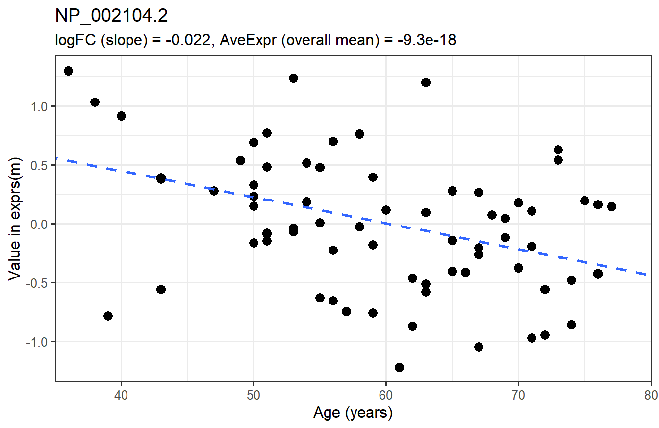
## NP_002104.2 -0.02214664 -9.315227e-18 -3.711539 4.238866e-04 0.5057768
## NP_002635.2 -0.05455354 -3.128810e-17 -4.266737 9.198715e-05 0.5057768
## NP_003286.1 0.01432046 -6.938894e-18 3.801188 3.156548e-04 0.5057768
## NP_005657.1 -0.02421416 8.935014e-18 -3.721088 4.108575e-04 0.5057768
## NP_006387.1 0.01887213 -1.368768e-17 3.637909 5.384586e-04 0.5057768
## NP_006535.1 -0.01271186 -3.041707e-18 -3.698719 4.420011e-04 0.5057768
## B
## NP_002104.2 -1.3815025
## NP_002635.2 0.3619802
## NP_003286.1 -1.1003103
## NP_005657.1 -1.3517595
## NP_006387.1 -1.6091557
## NP_006535.1 -1.4213571When accounting for differences due to Batch, no features have a significant linear relationship with AGE. Again, we will show a graphical representation of the top feature.