1.1 Prepare MS/MS Identifications

1.1.1 Read MS-GF+ Data

The first step in the preparation of the MS/MS identifications is to fetch the data. This can either be obtained from PNNL’s DMS or from a local folder. If working with the DMS, use PNNL.DMS.utils::read_msgf_data_from_DMS; otherwise, use PlexedPiper::read_msgf_data.

## Get MS-GF+ results from local folder - not run
# Get file path
path_to_MSGF_results <- "path_to_msgf_results"
# Read MS-GF+ data from path
msnid <- read_msgf_data(path_to_MSGF_results)

## Get MS-GF+ results from DMS
data_package_num <- 3442 # global proteomics
msnid <- read_msgf_data_from_DMS(data_package_num) # global proteomics

Normally, this would display a progress bar in the console as the data is being fetched. However, the output was suppressed to save space. We can view a summary of the MSnID object with the show() function.

show(msnid)

## MSnID object
## Working directory: "."
## #Spectrum Files:  48 
## #PSMs: 1156754 at 31 % FDR
## #peptides: 511617 at 61 % FDR
## #accessions: 128378 at 98 % FDR

This summary tells us that msnid consists of 4 spectrum files (datasets), and contains a total of 1,156,754 peptide-spectrum-matches (PSMs), 511,617 total peptides, and 128,378 total accessions (proteins). The reported FDR is the empirical false-discovery rate, which is calculated as the ratio of the number of unique decoy to unique non-decoy PSMs, peptides, or accessions.

1.1.2 Correct Isotope Selection Error

Carbon has two stable isotopes: \(^{12}\text{C}\) and \(^{13}\text{C}\), with natural abundances of 98.93% and 1.07%, respectively (Berglund et al., 2011). That is, we expect that about 1 out of every 100 carbon atoms is naturally going to be a \(^{13}\text{C}\), while the rest are \(^{12}\text{C}\). In larger peptides with many carbon atoms, it is more likely that at least one atom will be a \(^{13}\text{C}\) than all atoms will be \(^{12}\text{C}\). In cases such as these, a non-monoisotopic ion will be selected by the instrument for fragmentation.

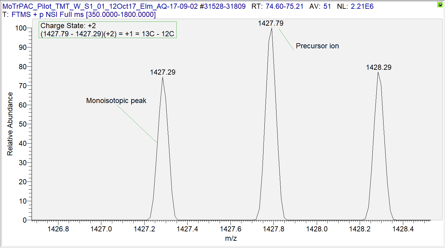
Figure 1.1: MS1 spectra with peak at non-monoisotopic precursor ion.

In Figure 1.1, the monoisotopic ion (m/z of 1427.29) is not the most abundant, so it is not selected as the precursor. Instead, the ion with a \(^{13}\text{C}\) in place of a \(^{12}\text{C}\) is selected for fragmentation. We calculate the mass difference between these two ions as the difference between the mass-to-charge ratios multiplied by the ion charge. In this case, the mass difference is 1 Dalton, or about the difference between \(^{13}\text{C}\) and \(^{12}\text{C}\). (More accurately, the difference between these isotopes is 1.0033548378 Da.) While MS-GF+ is still capable of correctly identifying these peptides, the downstream calculations of mass measurement error need to be fixed because they are used for filtering later on (Section 1.1.4). The correct_peak_selection function corrects these mass measurement errors, and Figure 1.2 shows the distribution of the absolute mass measurement errors (in PPM) before and after correction. This step influences the results of the peptide-level FDR filter.

# Correct for isotope selection error
msnid <- correct_peak_selection(msnid)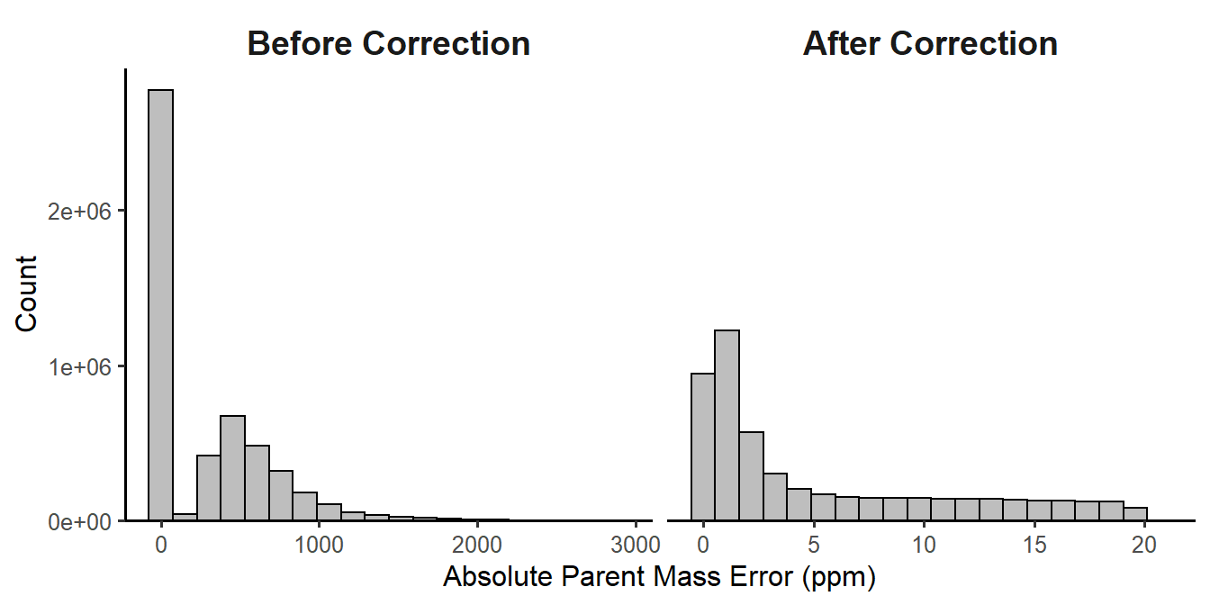

Figure 1.2: Histogram of mass measurement errors before and after correction.

1.1.3 Remove Contaminants

Now, we will remove contaminants such as the trypsin that was used for protein digestion. We can see which contaminants will be removed with accessions(msnid)[grepl("Contaminant", accessions(msnid))]. To remove contaminants, we use apply_filter with an appropriate string that tells the function what rows to keep. In this case, we keep rows where the accession does not contain “Contaminant”. We will use show to see how the counts change. This step is performed toward the beginning so that contaminants are not selected over other proteins in the filtering or parsimonious inference steps—only to be removed later on.

# Remove contaminants
msnid <- apply_filter(msnid, "!grepl('Contaminant', accession)")
show(msnid)

## MSnID object
## Working directory: "."
## #Spectrum Files:  48 
## #PSMs: 1155442 at 31 % FDR
## #peptides: 511196 at 61 % FDR
## #accessions: 128353 at 98 % FDR

We can see that the number of PSMs decreased by about 1300, peptides by ~400, and proteins by 25.

1.1.4 MS/MS ID Filter: Peptide Level

The next step is to filter the MS/MS identifications such that the empirical peptide-level FDR is less than some threshold and the number of identifications is maximized. We will use the \(-log_{10}\) of the PepQValue column as one of our filtering criteria and assign it to a new column in psms(msnid) called msmsScore. The PepQValue column is the MS-GF+ Spectrum E-value, which reflects how well the theoretical and experimental fragmentation spectra match; therefore, high values of msmsScore indicate a good match (see Figure 1.3).

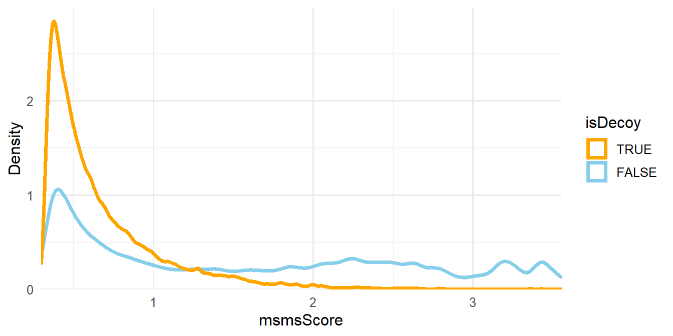
Figure 1.3: Density plot of msmsScore.

The other filtering criteria is the absolute deviation of the mass measurement error of the precursor ions in parts-per-million (ppm), which is assigned to the absParentMassErrorPPM column in psms(msnid) (see Figure 1.4).

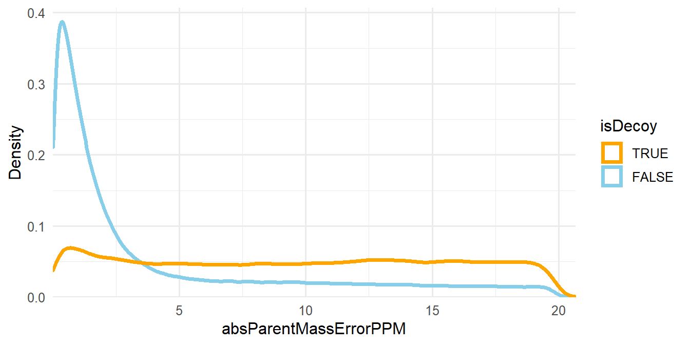
Figure 1.4: Density plot of absParentMassErrorPPM.

These new columns msmsScore and absParentMassErrorPPM are generated automatically by filter_msgf_data, so we don’t need to worry about creating them ourselves.

# 1% FDR filter at the peptide level
msnid <- filter_msgf_data(msnid, level = "peptide", fdr.max = 0.01)
show(msnid)

## MSnID object
## Working directory: "."
## #Spectrum Files:  48 
## #PSMs: 471295 at 0.46 % FDR
## #peptides: 96663 at 1 % FDR
## #accessions: 27098 at 9.1 % FDR

We can see that filtering drastically reduces the number of PSMs, and the empirical peptide-level FDR is now 1%. However, notice that the empirical protein-level FDR is still fairly high.

1.1.5 MS/MS ID Filter: Protein Level

(This step can be skipped if the final cross-tab will be at the peptide level.)

Now, we need to filter proteins so that the FDR is at most 1%. For each protein, we divide the number of associated peptides by its length and multiply this value by 1000. This new peptides_per_1000aa column is used as the filter criteria (Figure 1.6).

We will need the lengths of each protein, which can be obtained from the FASTA (pronounced FAST-AYE) file that contains the protein sequences used in the database search. The first three entries of the FASTA file are shown in Figure 1.5.

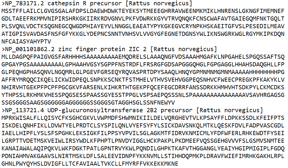
Figure 1.5: First three entries of the FASTA file.

The path to the FASTA file can be specified as a local file path or it can be obtained with PNNL.DMS.utils::path_to_FASTA_used_by_DMS. We will use the latter method.

## Get path to FASTA file from local folder - not run
path_to_FASTA <- "some_folder/name_of_fasta_file.fasta"

## Get path to FASTA file from DMS
path_to_FASTA <- path_to_FASTA_used_by_DMS(data_package_num)

# Compute number of peptides per 1000 amino acids
msnid <- compute_num_peptides_per_1000aa(msnid, path_to_FASTA)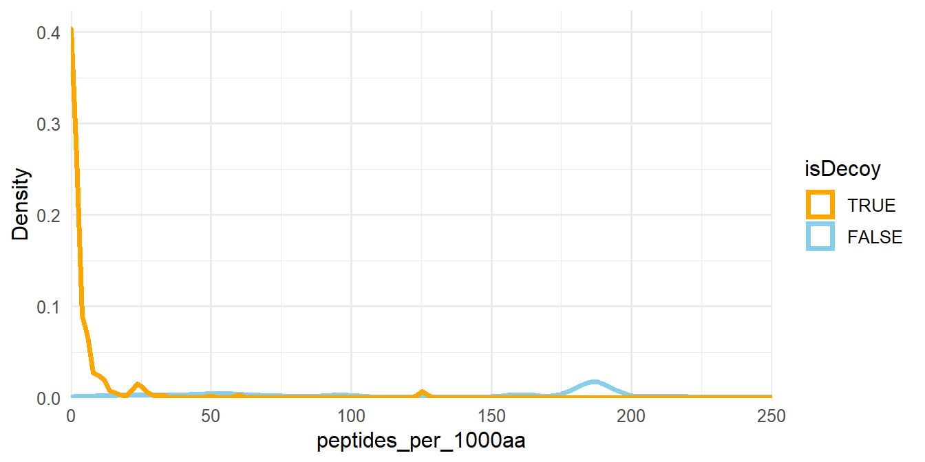

Figure 1.6: Density plot of peptides_per_1000aa. The plot area has been zoomed in.

Now, we filter the proteins to 1% FDR.

# 1% FDR filter at the protein level
msnid <- filter_msgf_data(msnid, level = "accession", fdr.max = 0.01)
show(msnid)

## MSnID object
## Working directory: "."
## #Spectrum Files:  48 
## #PSMs: 464788 at 0.17 % FDR
## #peptides: 92176 at 0.34 % FDR
## #accessions: 15629 at 0.98 % FDR

1.1.6 Inference of Parsimonious Protein Set

The situation when a certain peptide sequence matches multiple proteins adds complication to the downstream quantitative analysis, as it is not clear which protein this peptide is originating from. There are common ways for dealing with this. One is to simply retain uniquely-matching peptides and discard shared peptides (unique_only = TRUE). Alternatively, assign the shared peptides to the proteins with the most peptides (unique_only = FALSE). If there is a choice between multiple proteins with equal numbers of peptides, the shared peptides are assigned to the first protein according to alphanumeric order. It is an implementation of the greedy set cover algorithm. See ?MSnID::infer_parsimonious_accessions for more details.

There is no single best approach for handling duplicate peptides. Some choose to not do anything and allow peptides to map to multiple proteins. With parsimonious inference, we make the assumption that proteins with more mapped peptides are more confidently identified, so we should assign shared peptides to them; however, this penalizes smaller proteins with fewer peptides. Think carefully before deciding which approach to use.

Note: This step could be done prior to filtering at the accession level, but if peptides are assigned to a low-confidence protein, and that protein is removed during filtering, those peptides will be lost. Instead, it is better to filter to the set of confidently-identified proteins and then determine the parsimonious set.

# Inference of parsimonious protein set
msnid <- infer_parsimonious_accessions(msnid, unique_only = FALSE)
show(msnid)

## MSnID object
## Working directory: "."
## #Spectrum Files:  48 
## #PSMs: 451568 at 0.16 % FDR
## #peptides: 90639 at 0.28 % FDR
## #accessions: 5247 at 1.1 % FDR

Notice that the protein-level FDR increased slightly above the 1% threshold. In this case, the difference isn’t significant, so we can ignore it.

Note: If the peptide or accession-level FDR increases significantly above 1% after inference of the parsimonious protein set, consider lowering the FDR cutoff (for example, to 0.9%) and redoing the previous processing steps. That is, start with the MSnID prior to any filtering and redo the FDR filtering steps.

1.1.7 Remove Decoy PSMs

The final step in preparing the MS/MS identifications is to remove the decoy PSMs, as they were only needed for the FDR filters. We use the apply_filter function again and only keep entries where isDecoy is FALSE.

# Remove Decoy PSMs
msnid <- apply_filter(msnid, "!isDecoy")
show(msnid)

## MSnID object
## Working directory: "."
## #Spectrum Files:  48 
## #PSMs: 450857 at 0 % FDR
## #peptides: 90382 at 0 % FDR
## #accessions: 5191 at 0 % FDR

After processing, we are left with 450,928 PSMs, 90,411 peptides, and 5,201 proteins. Table 1.1 shows the first 6 rows of the processed MS-GF+ output.

Table 1.1: First 6 rows of the processed MS-GF+ results.
Dataset	ResultID	Scan	FragMethod	SpecIndex	Charge	PrecursorMZ	DelM	DelM_PPM	MH	peptide	Protein	NTT	DeNovoScore	MSGFScore	Rank_MSGFDB_SpecEValue	QValue	PepQValue	accession	calculatedMassToCharge	chargeState	experimentalMassToCharge	isDecoy	spectrumFile	spectrumID	pepSeq	msmsScore	absParentMassErrorPPM	peptides_per_1000aa
MoTrPAC_Pilot_TMT_W_S1_07_12Oct17_Elm_AQ-17-09-02	1862	27707	HCD	324	2	928.541	-0.001	-0.526	1856.075	R.AAAAAAAAAAAAAAGAAGK.E	NP_113986.1	2	285	282	1	0.000	0.000	NP_113986.1	928.541	2	928.541	FALSE	MoTrPAC_Pilot_TMT_W_S1_07_12Oct17_Elm_AQ-17-09-02	27707	AAAAAAAAAAAAAAGAAGK	Inf	0.589	24.938
MoTrPAC_Pilot_TMT_W_S1_07_12Oct17_Elm_AQ-17-09-02	4192	27684	HCD	906	3	619.363	-0.002	-0.887	1856.075	R.AAAAAAAAAAAAAAGAAGK.E	NP_113986.1	2	156	144	1	0.000	0.000	NP_113986.1	619.363	3	619.363	FALSE	MoTrPAC_Pilot_TMT_W_S1_07_12Oct17_Elm_AQ-17-09-02	27684	AAAAAAAAAAAAAAGAAGK	Inf	0.991	24.938
MoTrPAC_Pilot_TMT_W_S2_06_12Oct17_Elm_AQ-17-09-02	26263	27336	HCD	5187	3	619.363	0.000	0.197	1856.075	R.AAAAAAAAAAAAAAGAAGK.E	NP_113986.1	2	118	85	1	0.000	0.000	NP_113986.1	619.363	3	619.363	FALSE	MoTrPAC_Pilot_TMT_W_S2_06_12Oct17_Elm_AQ-17-09-02	27336	AAAAAAAAAAAAAAGAAGK	Inf	0.091	24.938
MoTrPAC_Pilot_TMT_W_S2_07_12Oct17_Elm_AQ-17-09-02	1471	27096	HCD	415	3	619.363	-0.001	-0.591	1856.075	R.AAAAAAAAAAAAAAGAAGK.E	NP_113986.1	2	157	156	1	0.000	0.000	NP_113986.1	619.363	3	619.363	FALSE	MoTrPAC_Pilot_TMT_W_S2_07_12Oct17_Elm_AQ-17-09-02	27096	AAAAAAAAAAAAAAGAAGK	Inf	0.684	24.938
MoTrPAC_Pilot_TMT_W_S2_05_12Oct17_Elm_AQ-17-09-02	28664	10441	HCD	4849	2	586.832	-0.001	-0.728	1172.659	R.AAAAADLANR.S	NP_001007804.1	2	124	124	1	0.002	0.003	NP_001007804.1	586.833	2	586.832	FALSE	MoTrPAC_Pilot_TMT_W_S2_05_12Oct17_Elm_AQ-17-09-02	10441	AAAAADLANR	2.480	0.746	34.755
MoTrPAC_Pilot_TMT_W_S1_24_12Oct17_Elm_AQ-17-09-02	41775	8033	HCD	7889	2	831.447	0.000	0.000	1661.886	G.AAAAAEAESGGGGGK.K	NP_001128630.1	1	176	76	1	0.001	0.003	NP_001128630.1	831.447	2	831.447	FALSE	MoTrPAC_Pilot_TMT_W_S1_24_12Oct17_Elm_AQ-17-09-02	8033	AAAAAEAESGGGGGK	2.583	0.106	579.815

References

Berglund, M. and Wieser, M. E., Isotopic Compositions of the Elements 2009 (IUPAC Technical Report), Pure and Applied Chemistry, vol. 83, no. 2, pp. 397–410, accessed February 12, 2022, from https://www.degruyter.com/document/doi/10.1351/PAC-REP-10-06-02/html, January 2011. DOI: 10.1351/PAC-REP-10-06-02